The Finger Tree

An array indexes in O(1) and cannot insert in the middle. A deque is cheap at both ends and cannot index. A balanced search tree splits in O(log n) but pays that logarithm even to read the first element, because the first element is a leaf.

The finger tree of Hinze and Paterson gives amortized O(1) at both ends, split and index at position i in O(log(min(i, n − i))), and concatenation in O(log(min(m, n))). The rest of this chapter is how, working from the datatype outward.

Three cases: empty, one element, or a deep node holding a prefix, a middle, and a suffix. The prefix and suffix are digits of one to four elements. The middle is a finger tree of nodes, where a node is a 2-3 branch.

data FingerTree a
  = Empty
  | Single a
  | Deep (Digit a) (FingerTree (Node a)) (Digit a)

data Digit a = One a | Two a a | Three a a a | Four a a a a
data Node  a = Node2 a a | Node3 a a a

Read the third constructor carefully: the middle of a FingerTree a is not a FingerTree a. It is a FingerTree (Node a) — a tree whose elements are pairs or triples of the level above.

That nesting is what makes the shape work. At the top level the digits hold plain elements. One level down they hold Node a, so each slot covers two or three elements. Two levels down they hold Node (Node a), covering four to nine. At depth k, one slot covers between 2^k and 3^k elements.

So a tree of n elements has a spine of depth O(log n), and the elements nearest each end sit in the outermost digits at depth zero. This is the ordinary 2-3 tree turned inside out: instead of a root with leaves below, the two ends are on top and the middle is buried. The type is polymorphically recursive, so the depth is tracked by the compiler rather than by a field in the node.

Pushing on the left reduces to four cases, and only the last one recurses.

pushL x Empty      = Single x
pushL x (Single y) = Deep (One x) Empty (One y)

pushL x (Deep (Four a b c d) m sf) =           -- prefix is full
    Deep (Two x a) (pushL (Node3 b c d) m) sf

pushL x (Deep pr m sf) =                       -- prefix has room
    Deep (cons x pr) m sf

The last case allocates one digit and one Deep node and returns. No recursion, no traversal, and no dependence on the size of the tree — pushing onto a sequence of ten and one of ten million run the same three instructions.

When the prefix already holds four, the push cannot extend it. Three of the four are packed into a Node3 and pushed onto the middle tree — which is a tree of Node a, so a Node3 b c d is exactly one of its elements. The prefix is left holding two: the incoming x and the a that stayed behind.

That recursive push can itself hit a full prefix one level down and cascade, so a single push is O(log n) in the worst case. Note what the cascade leaves behind: every level it touches ends with a two-element prefix. A digit of two is two pushes away from overflowing again, which is the fact the amortized argument runs on.

Reading from the left is the same structure in reverse. The interesting case is a prefix that runs empty, which has to borrow from the middle.

viewL Empty          = Nil
viewL (Single x)     = Cons x Empty
viewL (Deep pr m sf) = Cons (head pr) (deepL (tail pr) m sf)

deepL [] m sf = case viewL m of        -- prefix now empty
    Nil       -> fromDigit sf          -- middle empty too
    Cons n m' -> Deep (nodeToDigit n) m' sf
deepL pr m sf = Deep pr m sf

Borrowing pulls one Node off the middle and unpacks it with nodeToDigit, turning a Node3 into a three-element digit. One recursive step refills the prefix with three elements, so the next two pops are local again.

Call a digit safe at sizes two and three, and dangerous at one and four. Only a dangerous digit forces the recursive case: four overflows on a push, one underflows on a pop.

An operation on a dangerous digit leaves it safe — the overflow leaves two, the borrow leaves three — so the next operation at that level is guaranteed cheap. Assign one credit to each dangerous digit on the spine and the recursive step pays for itself out of the credit it releases, giving O(1) amortized per push or pop. The prefix and suffix are analysed independently, so both ends are cheap at once.

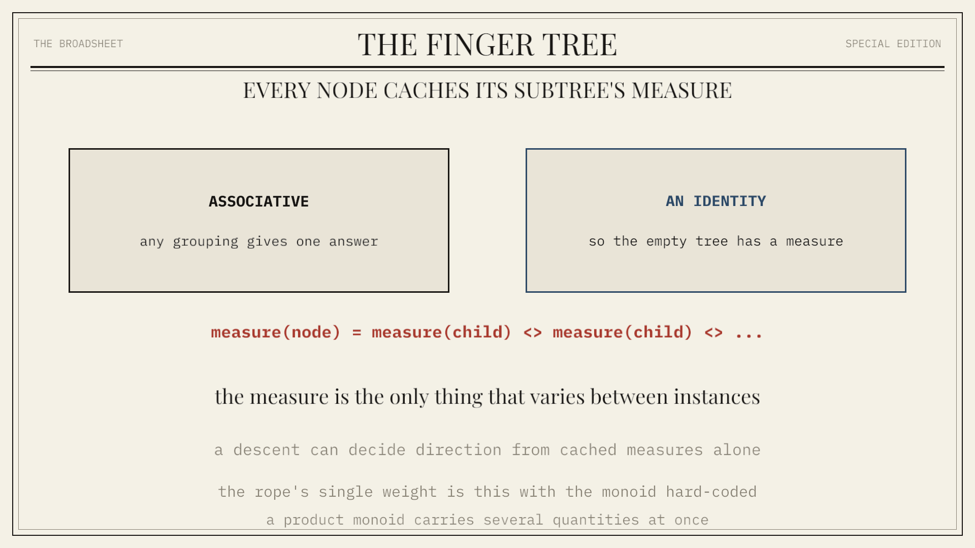
Every node stores a cached summary of its subtree. The summary type must be a monoid so that the tree can combine children in whatever grouping its shape has and get the same answer.

class Monoid v => Measured v a where
    measure :: a -> v

-- a node stores its measure; it is never recomputed
data Node v a = Node2 v a a | Node3 v a a a

instance Measured v (Node v a) where
    measure (Node2 v _ _)   = v
    measure (Node3 v _ _ _) = v

node3 a b c = Node3 (measure a <> measure b <> measure c) a b c

The cache is maintained by the smart constructor node3, so no operation has to remember to update it. A Deep node caches its total the same way, which is what lets a descent choose a direction by reading three numbers instead of visiting a subtree.

The base case of every positional query is a linear scan over at most four elements, accumulating the measure as it goes.

splitDigit p i [x]      = ([], x, [])
splitDigit p i (x:xs)
  | p i'      = ([], x, xs)        -- x is the element
  | otherwise = let (l, y, r) = splitDigit p i' xs
                in (x:l, y, r)
  where i' = i <> measure x

The predicate p is applied to the measure accumulated up to and including x, never to x itself. It must be monotone: false while the accumulated measure is small, true from some point onward. Given that, the first position where it flips is the answer, and four steps at most find it.

The whole structure hangs off one recursive function. It tests prefix, then middle, then suffix, and enters the first region whose accumulated measure satisfies the predicate.

splitTree p i (Deep pr m sf)
  | p (i <> measure pr) =                       -- in the prefix
      let (l, x, r) = splitDigit p i pr
      in Split (fromList l) x (deepL r m sf)

  | p (i <> measure pr <> measure m) =          -- in the middle
      let (ml, n, mr) = splitTree p (i <> measure pr) m
          i'          = i <> measure pr <> measure ml
          (l, x, r)   = splitDigit p i' (nodeToDigit n)
      in Split (deepR pr ml l) x (deepL r mr sf)

  | otherwise =                                 -- in the suffix
      let (l, x, r) = splitDigit p (i <> measure pr <> measure m) sf
      in Split (deepR pr m l) x (fromList r)

The middle case recurses one level down, finds a Node, then unpacks that node into a digit and scans it. Each level does constant work and the recursion is entered from whichever end is nearer, giving O(log(min(i, n − i))).

With splitTree in hand, the operations a sequence type normally implements separately are each one line. Measure every element as size 1 under addition, so the accumulated measure is a count:

splitAt i t = let Split l x r = splitTree (> i) mempty t in (l, pushL x r)
index    i t = let Split _ x _ = splitTree (> i) mempty t in x
takeUntil p t = fst (split p t)
dropUntil p t = snd (split p t)

Nothing here inspects an element or knows what the measure means. Change the predicate and the same descent answers a different question — which is the whole reason the split is written against accumulated measures rather than against indices.

Concatenation keeps the outer digits of both trees and pushes the inner ones into the recursion as a list of loose elements.

app3 Empty ts xs = foldr pushL xs ts
app3 xs ts Empty = foldl pushR xs ts
app3 (Deep pr1 m1 sf1) ts (Deep pr2 m2 sf2) =
    Deep pr1 (app3 m1 (nodes (sf1 ++ ts ++ pr2)) m2) sf2

nodes [a,b]      = [Node2 a b]
nodes [a,b,c]    = [Node3 a b c]
nodes [a,b,c,d]  = [Node2 a b, Node2 c d]
nodes (a:b:c:xs) = Node3 a b c : nodes xs

The middle argument ts holds at most eight elements — four from sf1, four from pr2 — and nodes packs them into 2-3 nodes for the next level down. Both spines are descended together and the recursion stops when the shorter runs out, so the cost is O(log(min(m, n))).

The code above never mentions what v is. Fix the monoid and the same tree becomes a different structure:

measure _ = 1        under (+)      -- random-access sequence
measure x = prio x   under max      -- priority queue
measure x = (1, prio x)             -- priority search queue
measure x = high x   under max      -- interval tree
measure x = key x    under lastKey  -- ordered search tree

For the priority queue, splitTree (>= maxPrio) descends to the highest-priority element in O(log n) while leaving the sequence in position order — something a binary heap cannot do, because a heap's array order is not the element order.

The amortized argument assumes each version is used once. Take the version one push away from an overflow, and push onto it repeatedly: each push pays the full cascade, and the credit banked once is spent many times. The bound fails exactly as described for persistent structures generally.

The repair is that the middle of a Deep node is a lazy suspension rather than a materialised tree. The first forcing runs the cascade and memoises it; every other version sharing that suspension reads the cached result. The payment happens at most once however many versions exist, so O(1) amortized holds under arbitrary reuse. In a strict language the same shape gives worst-case O(log n) at the ends unless scheduling is added.

Every element sits behind a chain of pointers, every node carries a cached measure beside its children, and every operation allocates. Against a flat array, indexing is a logarithmic pointer chase rather than one load, and iteration touches many separately allocated nodes.

The digits recover part of this: the outermost one to four elements at each end are directly reachable, which is why the ends are genuinely fast rather than merely logarithmic. The middle gets no such help. A workload that only indexes randomly is paying for the tree without using anything it provides — and if the workload only pushes and pops at the ends, a growable ring buffer is smaller and faster.

Haskell's containers package implements Data.Sequence as a finger tree measured by size, and it is the standard general-purpose sequence in that ecosystem; containers is a GHC boot library, so the compiler's own build depends on it. The fingertree package exposes the measure as a public parameter and ships Data.IntervalMap.FingerTree and Data.PriorityQueue.FingerTree, both the same tree with different monoids rather than separate implementations.

Beyond Haskell and direct ports, the sources reviewed for this chapter do not identify a widely deployed production system documenting a finger tree. The structure's influence has been as a design — the annotated, splittable, concatenable tree — which reappears in rope implementations that cache summaries at internal nodes without adopting the digit-and-spine shape.

A finger tree is a 2-3 tree turned inside out, so both ends sit at the top and the middle is buried under a spine of O(log n) levels. Digits of one to four elements absorb pushes and pops locally, and the safe-versus-dangerous accounting over digit sizes gives O(1) amortized at both ends.

Every node caches a monoidal measure, and one function — splitTree on a monotone predicate over accumulated measures — yields indexing, take, drop, priority selection, and interval search. Concatenation repacks at most eight loose elements per level and descends both spines together. The bounds survive version reuse only because the spine is a memoised suspension.