Big-O Notation

Algorithm analysis begins with a cost function such as T(n), where n measures the input and the value counts a chosen operation. The operation might be comparisons, array accesses, allocations, or bytes transferred. Wall-clock time is an observed consequence of those operations, not the mathematical input to the analysis.

The cost model must match the question. A comparison model is useful for sorting; an I/O model is more useful for an LSM tree. Big-O notation describes how the selected cost grows as the input grows.

Write f(n) = O(g(n)) when there are positive constants c and n₀ such that 0 ≤ f(n) ≤ c·g(n) for every n ≥ n₀. The constants allow the comparison to ignore a fixed multiplier and a finite prefix of small inputs.

Big-O is therefore an asymptotic upper bound. It does not mean that f equals g, and it need not be the tightest available bound. If f(n) = 3n + 8, then f(n) = O(n), O(n²), and many looser bounds are all true.

Big-Omega supplies the matching lower-bound relation: f(n) = Ω(g(n)) when f eventually stays above a positive constant multiple of g. Big-Theta combines both directions. f(n) = Θ(g(n)) means that g is an asymptotically tight bound for f.

For 3n + 8, the tight statement is Θ(n). Little-o and little-omega express strict separation: n = o(n log n), for example, because the ratio n / (n log n) tends to zero.

The variable n must identify what grows. For an array, it commonly counts elements. For a graph, a useful bound often needs both vertices and edges, such as O(V + E). An integer algorithm may depend on the number of input bits, ⌊log₂ x⌋ + 1, rather than on the numeric value x.

Collapsing several dimensions into one can hide the dominant resource. A Bloom filter is described by the number of inserted items, the number of bits, and the number of hash probes. State these parameters before comparing bounds.

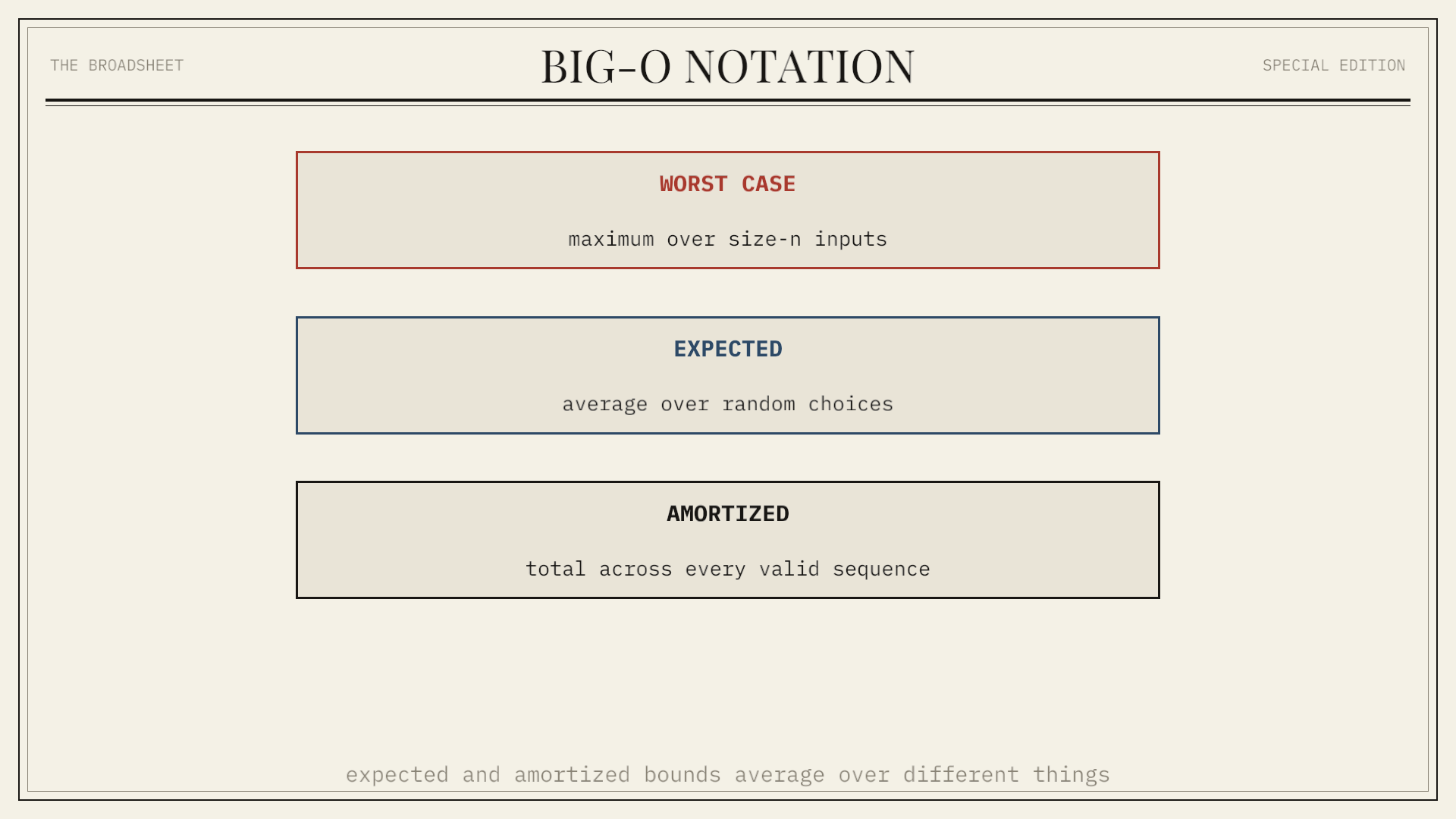
A complexity bound needs a qualifier. Worst-case cost takes the maximum over inputs of size n. Best-case cost takes the minimum. Average-case cost requires a probability distribution over inputs, while expected cost may instead average over the algorithm's own random choices.

Amortized cost averages across an operation sequence without assuming a random input. A treap has expected logarithmic height because of random priorities; a splay tree has amortized logarithmic operations because expensive restructurings are paid for across a sequence. These are different guarantees.

Common classes, from slower to faster growth, include O(1), O(log n), O(n), O(n log n), O(n²), O(cⁿ) for fixed c > 1, and O(n!). The ordering concerns sufficiently large inputs; constants can reverse measured performance over a finite range.

A van Emde Boas tree illustrates why parameters matter. Its O(log log U) operation bound uses universe size U, while its classic space cost is O(U). A faster time class does not settle the engineering choice.

For T(n) = 4n² + 20n + 600, the quadratic term eventually dominates, so T(n) = Θ(n²). Multiplying by a fixed constant or adding a lower-order term does not change the asymptotic class.

This simplification is valid only after the counted resource and computational model are fixed. A cache miss and an integer addition do not have the same latency, and a large constant can matter at every input size a system will encounter. Asymptotic analysis complements measurement; it does not replace it.

Sequential phases add their costs. A pass taking Θ(n) followed by a sort taking Θ(n log n) has total cost Θ(n log n). Nested loops multiply iteration counts when the inner work repeats independently for every outer iteration.

Bounds should follow the actual iteration space. A triangular loop whose inner index runs from 0 to the outer index performs 1 + 2 + … + n = Θ(n²) iterations. Two adjacent loops of n iterations perform 2n = Θ(n), not Θ(n²).

An operation is commonly logarithmic when each step reduces the remaining problem by a fixed factor. Halving an interval reaches size one after ⌈log₂ n⌉ steps. Changing the logarithm base multiplies the result by a constant, so asymptotic notation writes Θ(log n) without a base.

Balanced search structures use this reduction in tree form. An AVL tree keeps its height logarithmic, so a root-to-leaf search takes O(log n) comparisons in the worst case.

The same notation describes memory. Total space includes the input representation; auxiliary space counts only additional storage used by the algorithm. An in-place algorithm may use O(1) auxiliary space while still operating on an O(n) input.

Peak live memory is usually the relevant quantity. A recursive computation may allocate one frame per active call, so its auxiliary space follows recursion depth rather than the total number of calls.

A Big-O statement does not provide an exact runtime, a crossover point, or a latency distribution. It can also hide allocation patterns, parallelism, cache locality, network round trips, and numeric constants. Two Θ(n) procedures can behave differently on the same machine.

Use the bound to exclude growth rates that will not scale, then benchmark representative sizes and workloads. Report the model and qualifier with the result: O(log n) worst-case comparisons is more informative than “runs in logarithmic time.”

Big-O gives an eventual upper bound on a defined cost function. Big-Omega gives a lower bound, and Big-Theta gives a tight bound. Each statement depends on an input measure, a cost model, and a qualifier such as worst-case or expected.

Constants and lower-order terms disappear from the growth class, but they remain relevant to deployed performance. Asymptotic bounds describe scaling; measurements establish costs over the operating range.