Space Complexity

Space complexity describes how memory consumption grows with input size. A space function S(n) can count bytes, machine words, array cells, or another explicitly defined storage unit.

As with time complexity, the bound needs an input measure and a qualifier. A worst-case O(n) space bound means that every input of size n uses at most a constant multiple of n units beyond a sufficiently large threshold.

Total space includes the input representation. Auxiliary space counts additional memory allocated by the algorithm. A procedure that scans an array with two indices uses O(n) total space because the array exists, but only O(1) auxiliary space.

The distinction must be stated. “Uses constant space” usually means constant auxiliary space, not that the input occupies no memory.

Space complexity normally measures the maximum memory simultaneously live during execution. Allocating and releasing an n-element buffer ten times still has Θ(n) peak auxiliary space when only one buffer exists at a time.

Summing every allocation instead measures allocation volume, which affects allocator traffic and memory bandwidth but is not the standard space bound. Both measurements can matter, so name the one being reported.

A fixed number of counters, indices, pointers, and temporary values takes Θ(1) space under a fixed-width word model. The values may depend on n; the number of stored words does not.

For arbitrary-precision integers, a counter up to n needs Θ(log n) bits. Word-space and bit-space models can therefore produce different bounds. State the model when integer width is part of the problem.

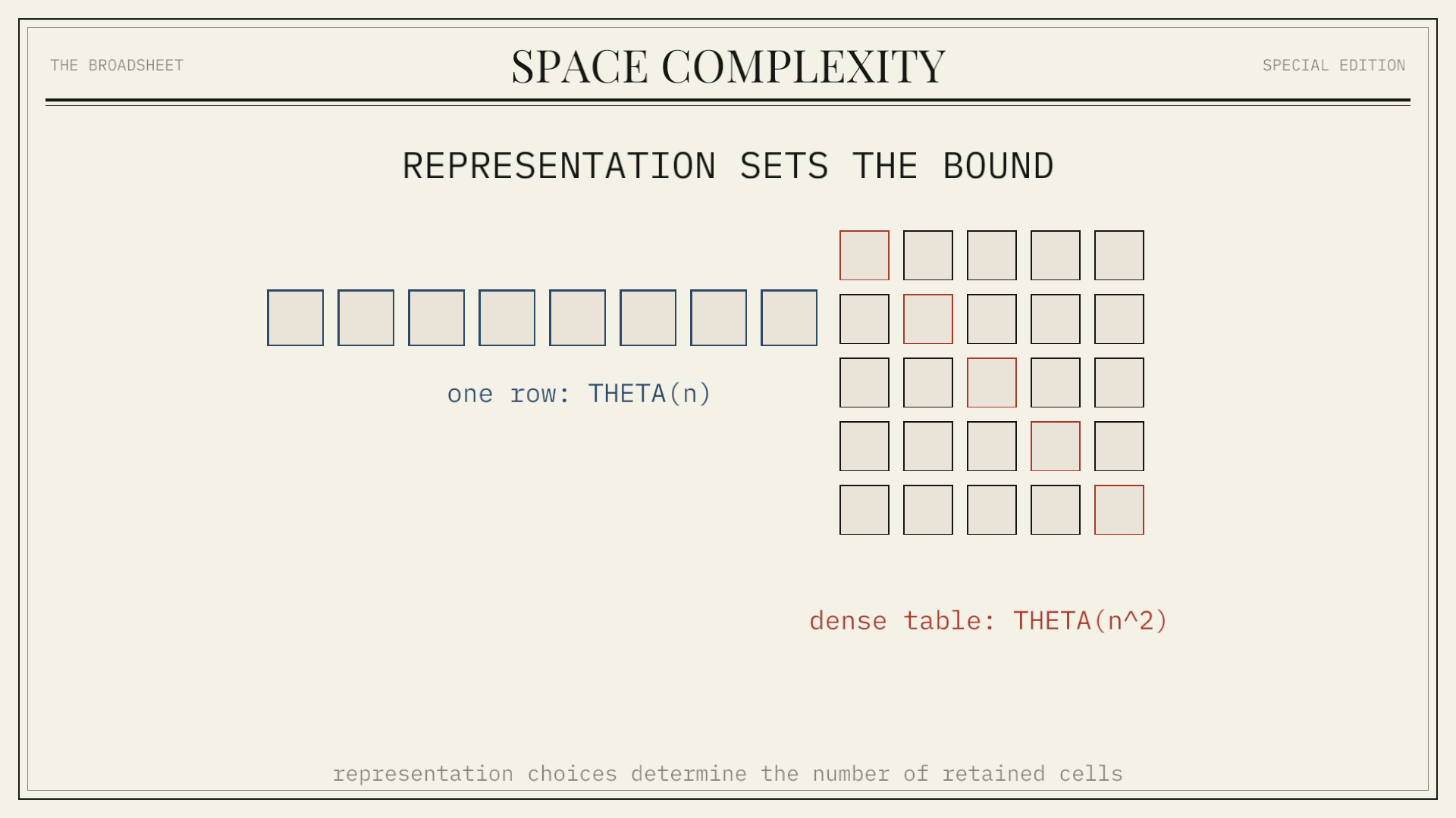
An array with one entry per input item uses Θ(n) space. A dense dynamic-programming table indexed by two input positions uses Θ(n²) cells when both dimensions have length n.

Representation changes the bound. An adjacency matrix uses Θ(V²) space, while adjacency lists use Θ(V + E). The latter saves memory for sparse graphs but still stores every vertex and edge.

Each active recursive call usually owns a stack frame containing return state, parameters, and local variables. If each frame is constant size, auxiliary stack space is proportional to the maximum recursion depth.

Recursive binary search has depth Θ(log n), while a recursive traversal of a skewed binary tree can reach Θ(n) depth if the tree is not balanced. Excessive depth can exhaust a runtime's finite thread stack.

The total number of recursive calls does not determine stack space. A traversal may visit Θ(n) nodes while retaining only one root-to-leaf path and a constant amount of state per level.

A balanced binary recursion can therefore take Θ(n) time and Θ(log n) stack space. If both child results or large per-call buffers remain live, those retained values must be added separately.

An algorithm is commonly called in place when it transforms its input using constant auxiliary storage. Swapping array elements with a fixed set of indices satisfies this definition.

The term has variations. Some definitions allow O(log n) stack frames, and stable in-place rearrangement may require more complex algorithms than unstable rearrangement. Report the actual bound instead of relying on the label alone.

Additional memory can remove repeated work. A prefix-sum array uses Θ(n) storage to answer range-sum queries in Θ(1) time. Memoization stores previously computed states to avoid recomputing overlapping subproblems.

The reverse trade is also common. A dynamic program that depends only on the previous row can replace an Θ(n²) table with two Θ(n) rows, but discarded states are no longer available for reconstructing a full solution path.

An object becomes logically dead when the program can no longer use it, but a garbage-collected runtime may reclaim its storage later. Heap capacity, retained live objects, and temporary allocation volume are different measurements.

Asymptotic analysis usually counts live reachable storage under an abstract reclamation model. Production profiling must also inspect retention, collector scheduling, object headers, fragmentation, and the peak resident set.

An external-memory algorithm separates main memory from disk or other block storage. Its analysis may bound internal memory M, block size B, and the number of block transfers rather than treating all bytes as equivalent.

Parallel algorithms need both per-worker and aggregate space. A computation using Θ(n) memory on each of p workers consumes Θ(pn) aggregate memory even though every worker reports the same local bound.

State whether a bound is total or auxiliary, and whether it counts words, bits, objects, or bytes. Include recursion stack space and retained intermediate results. For multiple inputs, preserve relevant parameters such as Θ(V + E).

Asymptotic notation does not supply concrete memory limits. After deriving the growth rate, measure object sizes and peak live memory for the runtime and workload that will execute the algorithm.

Space complexity bounds memory growth under a defined model. Total space includes the input; auxiliary space counts additional storage; peak live storage determines the standard bound.

Arrays, retained tables, recursion depth, and parallel replicas all contribute. In-place transformations reduce auxiliary storage, while caches and precomputed tables deliberately spend space to reduce time.