Recurrence Relations

A recurrence relation defines a quantity using values on smaller inputs. For a recursive algorithm, T(n) usually equals the cost of recursive calls plus the work performed in the current call.

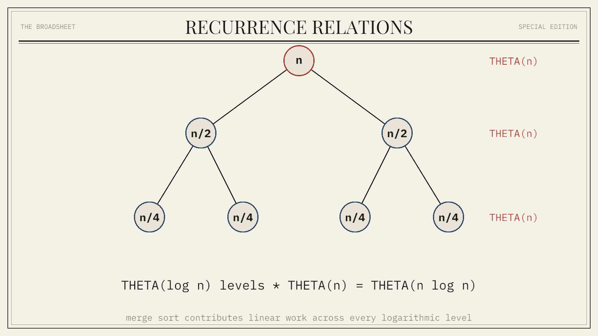
Merge sort makes two calls on half-size inputs and spends linear work splitting and merging, giving T(n) = 2T(n/2) + Θ(n). The recurrence records the program's call structure; solving it converts that structure into a bound in asymptotic notation.

A recurrence needs base cases. The merge-sort relation is completed by T(1) = Θ(1). Without a base case, the equation does not identify where recursion stops or what the leaves cost.

Analyses often assume that n is a power of two so every division is exact. Floors, ceilings, and uneven final subproblems usually change only constants for standard divide-and-conquer recurrences, but that claim must be justified rather than silently assumed.

Repeated substitution exposes a recurrence's pattern. For T(n) = T(n − 1) + n, expansion gives T(n) = T(n − 2) + (n − 1) + n, then continues to the base case.

The resulting sum is 1 + 2 + … + n = n(n + 1)/2, so T(n) = Θ(n²). Expansion is useful for discovering a candidate bound; induction can then prove it.

The substitution method guesses a bound and proves it by induction. To show T(n) = O(n log n) for merge sort, assume smaller inputs satisfy T(k) ≤ c k log k, substitute the assumption, and choose constants that absorb the non-recursive linear term.

A proof must include enough slack. Guessing only the leading term can fail when lower-order costs do not fit the induction. Strengthening the hypothesis, for example to T(n) ≤ c n log n + d n, often supplies the required margin.

A recursion tree places the original problem at the root, recursive subproblems at the next level, and base cases at the leaves. Each node is labelled with its non-recursive work. Summing a level and then summing the levels gives the total.

For merge sort, level i has 2ⁱ subproblems of size n/2ⁱ. Their merge work totals Θ(n) at every level. There are Θ(log n) levels, producing Θ(n log n) total work.

Not every recursion tree has equal work per level. In T(n) = 2T(n/2) + Θ(1), level costs grow geometrically toward the leaves, and the Θ(n) leaves dominate. In T(n) = 2T(n/2) + Θ(n²), costs shrink geometrically, so the root's Θ(n²) work dominates.

The important comparison is between the growth of the recursive population and the change in work per subproblem. The Master theorem formalizes that comparison for a common recurrence family.

The Master theorem handles recurrences of the form T(n) = aT(n/b) + f(n), where a is the number of equal-size subproblems, each subproblem has size n/b, and f(n) is the work outside recursion.

The term n^(log_b a) measures the leaf population. Compare f(n) with this term. The theorem then identifies whether the leaves, all levels together, or the root-side work determines the result.

If f(n) is polynomially smaller than n^(log_b a), recursive leaves dominate and T(n) = Θ(n^(log_b a)). If the terms match up to logarithmic factors, every level contributes comparable work and an additional logarithmic factor appears.

If f(n) is polynomially larger and satisfies the theorem's regularity condition, the non-recursive work dominates and T(n) = Θ(f(n)). The polynomial gaps and regularity condition are part of the theorem; comparing only the apparent exponents can produce an invalid result.

The standard Master theorem does not directly cover unequal subproblem sizes such as T(n) = T(n/3) + T(2n/3) + Θ(n), size-dependent branch counts, or recurrences such as T(n) = T(n − 1) + n.

A recurrence outside the theorem is not unsolvable. Expansion, substitution, recursion trees, characteristic equations, and the Akra–Bazzi method cover different forms. Select the method from the equation rather than forcing the equation into a memorized template.

The Akra–Bazzi theorem handles many divide-and-conquer recurrences with unequal subproblem fractions: T(x) = Σ aᵢT(bᵢx + hᵢ(x)) + g(x). First find p satisfying Σ aᵢbᵢᵖ = 1.

Under the theorem's conditions, the solution is Θ(xᵖ(1 + ∫₁ˣ g(u)/u^(p+1) du)). For T(n) = T(n/3) + T(2n/3) + Θ(n), p = 1, and the integral contributes Θ(log n), giving Θ(n log n).

Recurrences also describe data rather than runtime. The Fibonacci relation Fₙ = Fₙ₋₁ + Fₙ₋₂ is a linear recurrence with constant coefficients. Characteristic roots give a closed form and show exponential growth in n.

An AVL tree uses a related recurrence for the minimum number of nodes at height h: N(h) = 1 + N(h − 1) + N(h − 2). Its Fibonacci growth implies that height is O(log n).

An exact solution retains constants, floors, and lower-order terms. An asymptotic solution groups functions by growth rate. Algorithm analysis often needs only the latter because it is used to compare scaling behavior.

The required precision depends on the decision. Exact call counts can explain a measured threshold, while a tight Θ bound may be enough to reject an algorithm for large inputs. State which kind of solution has been established.

A recurrence follows recursive decomposition; it does not automatically capture costs shared across unrelated operations. A sequence of updates to a splay tree or union-find structure is usually handled by amortized analysis instead.

The distinction is structural. Recurrences split one computation into smaller computations. Amortized proofs distribute costs across time or state changes. Some analyses use both, but each equation must correspond to the work it claims to count.

A recurrence expresses a recursive algorithm's cost as subproblem costs plus local work. Base cases complete the definition. Expansion and recursion trees expose the sum; substitution proves a guessed bound.

The Master theorem solves equal-size divide-and-conquer forms, while Akra–Bazzi covers many unequal splits. When neither applies, use the recurrence's actual structure rather than discarding terms or applying a theorem outside its conditions.